
POWERUP builds explainable predictive models that connect molecular features to measured responses and applies those models to new samples.
Core workflow we will go over:
Prepare -> Train -> Predict -> Explain
For this quick tutorial, we will model CTNNB1 dependency and predict it in two held-out samples.
Load the example data
The package includes a compact example with 300 reference cell lines, 300 expression features, four dependency responses, and two held-out expression profiles used as prediction samples. The example is a demonstration subset of DepMap Public 26Q1 release. Please see Example data and provenance for its source data, construction, and acknowledgements.
expression_path <- system.file("extdata", "powerup_example_gene_expression.csv", package = "powerup")
dependency_path <- system.file("extdata", "powerup_example_gene_dependency.csv", package = "powerup")
user_path <- system.file("extdata", "powerup_example_user_matrix.csv", package = "powerup")

example_expression <- read.csv(expression_path, check.names = FALSE)
example_dependency <- read.csv(dependency_path, check.names = FALSE)
example_user <- read.csv(user_path, check.names = FALSE)

dim(example_expression)
## [1] 300 301
dim(example_dependency)## [1] 300 5
dim(example_user)## [1] 2 301We can inspect what these tables look like:
example_expression[1:3, 1:4]## ModelID ACSL5 ADAMTS1 ADGRF1
## 1 ACH-000007 7.06805 0.08750 4.64011
## 2 ACH-000009 4.57462 0.13586 0.21417
## 3 ACH-000015 0.08369 6.51186 0.03409
example_dependency[1:3, 1:4]## ModelID CTNNB1 ERBB2 FGFR1
## 1 ACH-000007 0.893872 0.863364 0.017890
## 2 ACH-000009 0.971451 0.981704 0.044951
## 3 ACH-000015 0.997204 0.263052 0.006654
example_user[, 1:4]## sample ACSL5 ADAMTS1 ADGRF1
## 1 ACH-000957 6.94027 0.11104 0.79013
## 2 ACH-002024 0.06129 0.00000 0.01245These are now ready to be passed to
prepare_powerup_data() for alignment and feature
selection.
FAQs
Q: How can I obtain the full data for training real models?
Download the full datasets from the DepMap portal.
Q: Can I use my own response data?
Yes. POWERUP can use compatible user-provided reference response matrices. See the function reference for the available settings and their intended use.
Q: How should I create expression data for my own samples?
For optimal alignment with the reference data, process your samples as comparably as possible to the reference data. This documentation includes instructions to achieve a close approximation of the DepMap expression data processing workflow for bulk RNA-seq. We also include the steps we followed for single-nucleus RNA-seq. For bulk RNA-seq, see Processing bulk RNA-seq inputs from FASTQ or BAM files. For single-cell or single-nucleus RNA-seq, see Generating pseudobulk from single-cell and single-nucleus RNA-seq.
Prepare the data
prepare_powerup_data() aligns the reference features and
measured responses with the samples that will receive predictions. Here
we select CTNNB1 as the single response we wish to model,
although you can fit models for multiple targets in a real run.
prepared <- prepare_powerup_data(
  gene_expression = example_expression,
  response = example_dependency,
  targets = "CTNNB1",
  user_matrix = example_user
)
## [powerup] target resolution summary requestedUnique=1 resolvedUnique=1 metadataNameMatches=0 canonicalFallbackMatches=1 looseMetadataFallbackResolved=0 exactMetadataMultipleMatches=0 unresolvedSkipped=0## [powerup] top-variable feature selection source=reference_matrix reason=user_selected_reference_source reference_samples=300 n_ranked_reference_features=300 n_user_available_features=300
dim(prepared$features_train)## [1] 300 301
dim(prepared$outcomes_train)## [1] 300 2
dim(prepared$features_user)## [1] 2 301We can get a table of perturbations we aim to model:
prepared$perturbations## # A tibble: 1 × 2
## modelKey perturbation
## <chr> <chr>
## 1 crispr_model_00001 CTNNB1This prepared object can then be passed directly to
fit_powerup_models().
Train a POWERUP model
fit_powerup_models() trains the perturbations selected
during data preparation. Because the prepared object contains only
CTNNB1 knockout response, one model is trained here.
models <- fit_powerup_models(prepared, seed = 123L)## [2026-08-24 02:40:36.357042 UTC] Training a model for CTNNB1 (1 of 1)
## [2026-08-24 02:40:37.650741 UTC] Cross-validation complete: r = 0.853 +/- 0.031 | R2 = 0.716 +/- 0.046 | RMSE = 0.19575 | CV best_nrounds median = 191 | n = 9
## [2026-08-24 02:40:38.304866 UTC] Uncertainty model complete: calibration factor = 1.569 | mean predicted 95% half-width = 0.259 | error CV best_nrounds median = 173
## [2026-08-24 02:40:38.306516 UTC] SHAP: preparing feature contributions
## [2026-08-24 02:40:38.306679 UTC] SHAP: calculating feature contributions
## [2026-08-24 02:40:38.336833 UTC] SHAP: predcontrib dimensions = 300 x 301
## [2026-08-24 02:40:38.337002 UTC] SHAP: feature dimensions = 300 x 300
## [2026-08-24 02:40:38.337131 UTC] SHAP: dimensions with bias = 300 x 301
## [2026-08-24 02:40:38.337259 UTC] SHAP: raw calculation complete
## [2026-08-24 02:40:38.337901 UTC] SHAP: compressing 300 samples x 300 features, keeping top 100 per sample
## [2026-08-24 02:40:38.340208 UTC] SHAP: compression 10% (30/300 samples)
## [2026-08-24 02:40:38.341696 UTC] SHAP: compression 20% (60/300 samples)
## [2026-08-24 02:40:38.343099 UTC] SHAP: compression 30% (90/300 samples)
## [2026-08-24 02:40:38.344506 UTC] SHAP: compression 40% (120/300 samples)
## [2026-08-24 02:40:38.345944 UTC] SHAP: compression 50% (150/300 samples)
## [2026-08-24 02:40:38.347357 UTC] SHAP: compression 60% (180/300 samples)
## [2026-08-24 02:40:38.348716 UTC] SHAP: compression 70% (210/300 samples)
## [2026-08-24 02:40:38.350075 UTC] SHAP: compression 80% (240/300 samples)
## [2026-08-24 02:40:38.351439 UTC] SHAP: compression 90% (270/300 samples)
## [2026-08-24 02:40:38.352811 UTC] SHAP: compression 100% (300/300 samples)
## [2026-08-24 02:40:38.352948 UTC] SHAP: combining compressed rows
## [2026-08-24 02:40:38.354954 UTC] SHAP: compression complete (300 samples x 241 retained feature columns)
## [2026-08-24 02:40:38.355139 UTC] Finalizing model object: CTNNB1
## [2026-08-24 02:40:38.355266 UTC] Model complete: CTNNB1Model performance can be summarized with:
summarize_models(models)## # A tibble: 1 × 13
## brd skipped r R2 rmse d_sensitivity d_specificity d_FPR d_PPV d_NPV
## <chr> <lgl> <dbl> <dbl> <dbl> <dbl> <dbl> <dbl> <dbl> <dbl>
## 1 CTNN… FALSE 0.853 0.716 0.196 0.832 0.973 0.0267 0.895 0.956
## # ℹ 3 more variables: d_accuracy <dbl>, n_terms <int>, mean_pred_sd <dbl>These cross-validation metrics are measured on held-out training samples, not on the new prediction samples. Higher correlation and R-squared and lower RMSE indicate better predictive performance. Model performance should be considered before interpreting individual predictions or their explanations. See Training and evaluating POWERUP models for the cross-validation, model-retention, and uncertainty procedures used during fitting.
Predict new samples
The same prepared object also contains the held-out prediction
samples. Pass it directly to add_powerup_predictions():
models <- add_powerup_predictions(models, prepared)Collect the predictions with:
predictions <- summarize_predictions(models)
predictions
## CTNNB1
## ACH-000957 0.9828395
## ACH-002024 0.1930624Each row is a sample and each column is a modeled response.
Explain each prediction
POWERUP calculates SHAP feature contributions alongside each
prediction. plot_contributions_to_sample() shows how
selected features move the model from its baseline prediction to the
final prediction for an explicitly chosen perturbation and sample.
The plotting function uses the same prepared object so
it can recover the original feature values for either training or user
samples. The default source parameter is
"training", which means the function will use the training
data. So here we set source = "user" because these two
samples were predicted from the user supplied data.
plot_contributions_to_sample(
  models,
  prepared,
  perturbations = "CTNNB1",
  samples = c("ACH-000957", "ACH-002024"),
  source = "user",
  n_columns = 1
)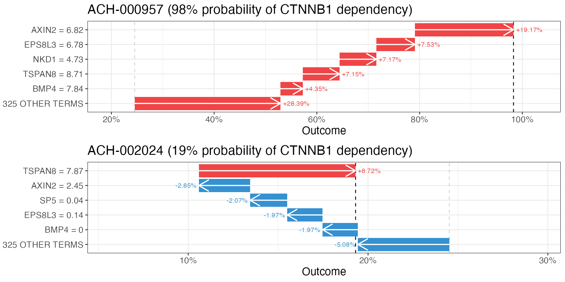
Each waterfall highlights the features that push that sample’s CTNNB1 essentiality prediction higher or lower.
Note that SHAP values explain the fitted model, not biological causality. A large contribution means that a feature strongly influenced the prediction; it does not show that changing the feature would change the response.
Summarize important features
We can visualize the strongest contributors to a given predictive model across the training cohort:
plot_top_contributors(
  models,
  data_to_use = "training",
  n_predictors = 10,
  n_columns = 1
)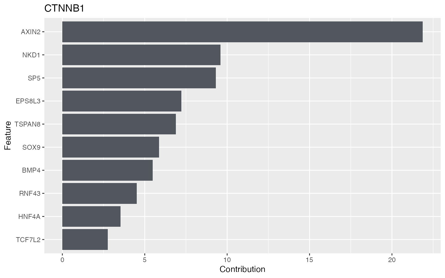
Using the same function, we can also visualize the top contributors
in the prediction cohort by setting
data_to_use = "new_data".
Next steps
If you need to generate a user expression matrix from paired-end RNA-seq FASTQs or BAMs, see Processing bulk RNA-seq inputs from FASTQ or BAM files. For single-cell or single-nucleus RNA-seq, see Generating pseudobulk from single-cell and single-nucleus RNA-seq. See Preparing data for POWERUP for feature selection, user samples, and held-out reference samples. The function reference provides additional options for model training, prediction, and explanation.
See Interpreting POWERUP results for guidance on model metrics and prediction outputs, and Explaining POWERUP predictions for detailed SHAP interpretation and explanation-path analysis. Continue with Experimental observations and posterior updating to incorporate experimental evidence.
Session information
## R version 4.4.2 (2024-10-31)
## Platform: aarch64-apple-darwin20
## Running under: macOS Sequoia 15.7.3
##
## Matrix products: default
## BLAS:   /Library/Frameworks/R.framework/Versions/4.4-arm64/Resources/lib/libRblas.0.dylib
## LAPACK: /Library/Frameworks/R.framework/Versions/4.4-arm64/Resources/lib/libRlapack.dylib;  LAPACK version 3.12.0
##
## locale:
## [1] en_US.UTF-8/en_US.UTF-8/en_US.UTF-8/C/en_US.UTF-8/en_US.UTF-8
##
## time zone: America/New_York
## tzcode source: internal
##
## attached base packages:
## [1] stats     graphics  grDevices utils     datasets  methods   base
##
## other attached packages:
## [1] powerup_1.0.95
##
## loaded via a namespace (and not attached):
##  [1] sass_0.4.9        utf8_1.2.4        future_1.34.0     generics_0.1.3
##  [5] tidyr_1.3.1       stringi_1.8.4     lattice_0.22-6    listenv_0.9.1
##  [9] digest_0.6.37     magrittr_2.0.3    evaluate_1.0.3    grid_4.4.2
## [13] fastmap_1.2.0     xgboost_3.2.1.1   jsonlite_2.0.0    Matrix_1.7-3
## [17] purrr_1.1.0       scales_1.3.0      codetools_0.2-20  textshaping_1.0.0
## [21] jquerylib_0.1.4   cli_3.6.5         rlang_1.1.6       parallelly_1.42.0
## [25] cowplot_1.1.3     munsell_0.5.1     withr_3.0.2       cachem_1.1.0
## [29] yaml_2.3.10       tools_4.4.2       parallel_4.4.2    dplyr_1.1.4
## [33] ggplot2_3.5.1     colorspace_2.1-1  rsample_1.2.1     globals_0.16.3
## [37] vctrs_0.6.5       R6_2.6.1          lifecycle_1.0.4   stringr_1.5.2
## [41] fs_1.6.5          htmlwidgets_1.6.4 ragg_1.5.1        furrr_0.3.1
## [45] pkgconfig_2.0.3   desc_1.4.3        gtable_0.3.6      pkgdown_2.2.0
## [49] pillar_1.10.1     bslib_0.9.0       glue_1.8.0        data.table_1.17.0
## [53] systemfonts_1.2.2 xfun_0.51         tibble_3.3.0      tidyselect_1.2.1
## [57] knitr_1.50        farver_2.1.2      htmltools_0.5.8.1 labeling_0.4.3
## [61] rmarkdown_2.29    compiler_4.4.2